Scientific Computing with JAX
A Case Study Evaluating Gravitational Lensing Likelihood
Presented at Durham HPC Days 2025.
JAX is a Python library that combines just-in-time (JIT) compilation with automatic differentiation, powered by XLA (Accelerated Linear Algebra compiler), to target multiple hardware architectures including CPU, GPU (NVIDIA, AMD, Intel, Apple), and Google TPU. While primarily designed for machine learning research, JAX presents compelling advantages for scientific computing in the HPC landscape.
As HPC increasingly depends on heterogeneous accelerators, JAX’s “write once, deploy anywhere” approach enables scientific libraries to efficiently utilize diverse computing resources. Python programmers familiar with array programming and other JIT solutions like Numba can transition to JAX with minimal code changes, allowing straightforward adoption. Additionally, automatic differentiation provides gradient calculations for optimization problems with minimal developer effort — automatically generating derivatives that would be prohibitively complex to implement manually, while enabling optimization algorithms to converge more rapidly with gradient information.
This presentation examines the adaptation of a likelihood function calculation from Numba to JAX in the context of gravitational lensing analysis of James Webb Space Telescope observations. The case study specifically addresses the convergence of AI/ML techniques with traditional scientific computing, highlighting performance gains, implementation challenges, and practical considerations when migrating existing scientific code to JAX’s programming model. We’ll discuss how JAX enables scalable processing across different HPC hardware resources while maintaining scientific accuracy and computational efficiency.
Below is a companion article to the Durham HPC Days 2025 talk on porting a gravitational lensing likelihood from Numba to JAX for JWST analysis. The slides and this article are generated from a single source, so everything that was on screen is here, together with an AI transcript of what was said around it.
Hello everyone. My name is Kolen Cheung, and I’m a Research Software Engineer at the University of Exeter. Today, I’m going to talk about a project I’ve worked on to adopt JAX for scientific computing, specifically a case study in evaluating gravitational lensing likelihood.
Motivations
Physics: revealing the nature of dark matter with the James Webb Space Telescope (JWST)
The project’s motivation is to probe the nature of dark matter with the James Webb Space Telescope (JWST). The science case is to investigate the low-mass region — below roughly \(10^{8.5} M_\odot\) — of dark matter substructures in our universe. This is the region where the well-established ΛCDM model and alternative dark matter models make statistically different predictions.
Substructures in that mass range are generally invisible, so we cannot observe them directly: we have to probe them via strong gravitational lensing. This was first demonstrated two years ago in James W. Nightingale et al.1 using Hubble Space Telescope (HST) data, so the natural next step is to take advantage of the 4+ wavebands and the high quality observations from JWST.
How? PyAutoLens
To do this, we use an existing package called PyAutoLens. It has two halves:
Mass modeling: parametric, non-linear, multi-phase models
Source reconstruction: linear, reconstructing unlensed light distribution via different kinds of meshes: rectangular, Delaunay, Voronoi
Log-likelihood function takes the output of (1) and computes its likelihood (where (2) is part of the calculation).
Key goal is to automate the whole process and apply it to large datasets.
The power of likelihood in theory
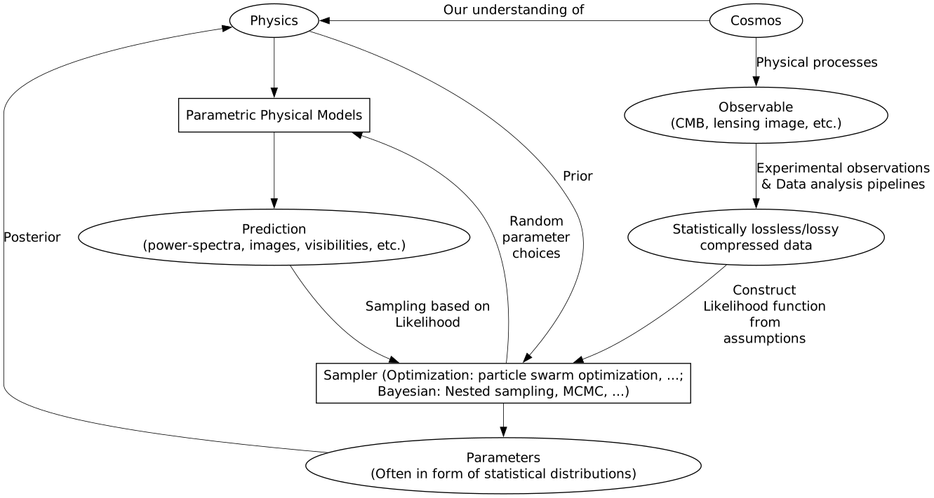
In cosmology, we cannot perform experiments; we only have one observable universe. All we can do is make observations and then use simulations to infer the parameters of physical models through statistical methods. That is the loop in the diagram above: physics gives us parametric models, models give us predictions, the cosmos gives us observables that our pipelines compress into data, and a sampler ties the two branches together through the likelihood function.
The power of likelihood in action
- 25 free parameters
- Lens Light (11): Sersic + Exponential
- Lens Mass (7): SIE + Shear
- Source Light (7): Sersic
PyAutoLens (via PyAutoFit) supports Nested sampling (Dynesty), MCMC (emcee), particle swarm optimization (PySwarms)
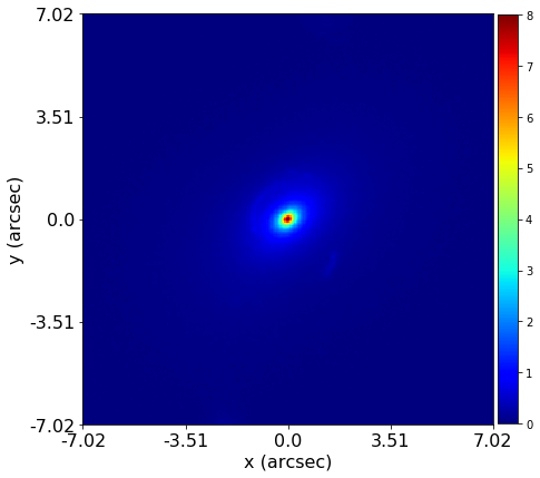
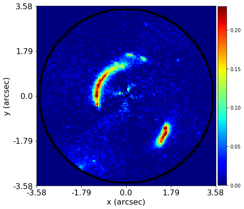
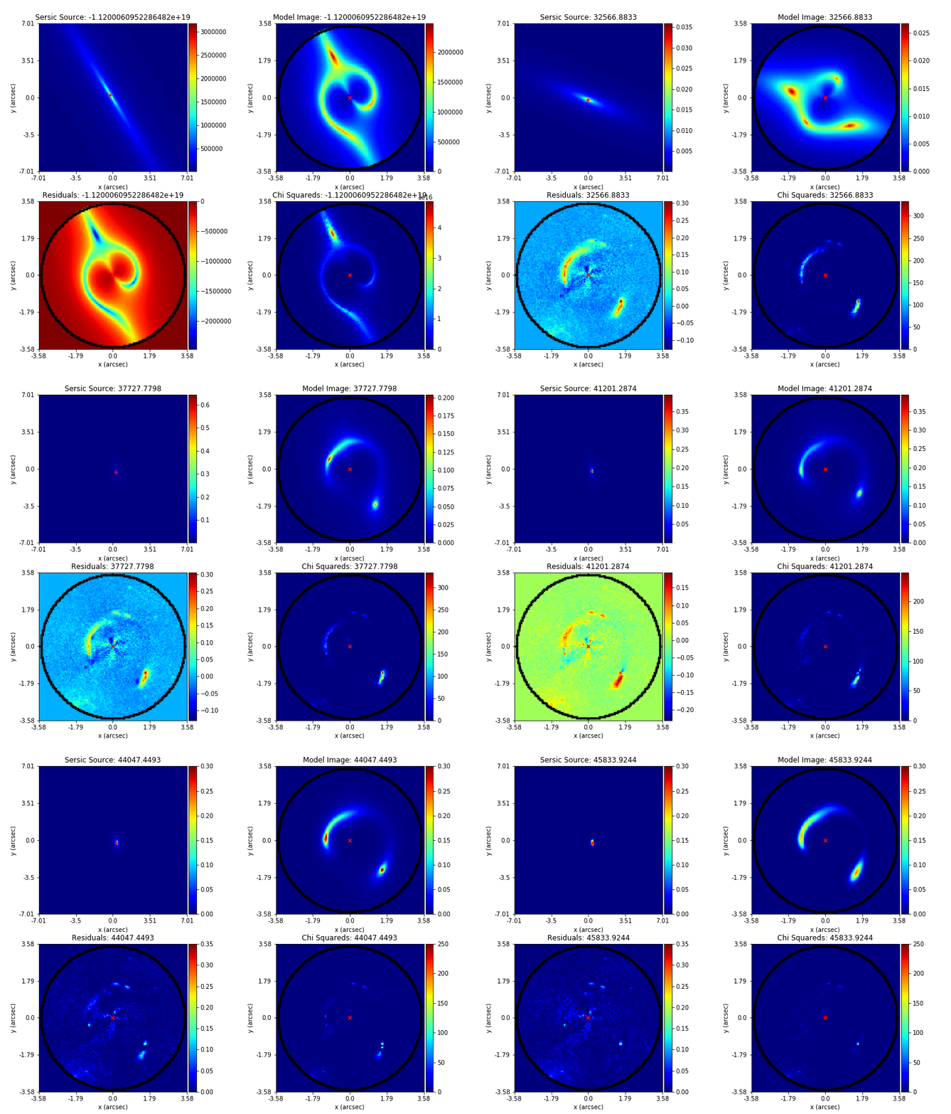
PyAutoLens uses a sampler to iterate and find the best solution. The goal is to find the mass profile that produces the observed image.
Computational challenges
However, there are computational challenges.
- PyAutoLens originally is implemented in Numba
- For single-band HST data, the image processing analysis of a single lens takes approximately 48 hours over 76 CPUs.
- image pixels: \(M \sim 10,000\)
- source image pixels: \(S \sim 2,000\)
- \(3\text{ s}\) for 1 iteration, \(O(100,000)\) iterations needed.
- For JWST’s 4x freq. bands, \(M \rightarrow 4M, S \rightarrow 4S\). Runtime: \(\sim 3\text{ s} \rightarrow 60\text{ s}\). I.e. \(\sim \times 20\)
That extra cost buys us something, though: because JWST provides data across multiple frequency bands, we get colour information that helps guide the model to better solutions.
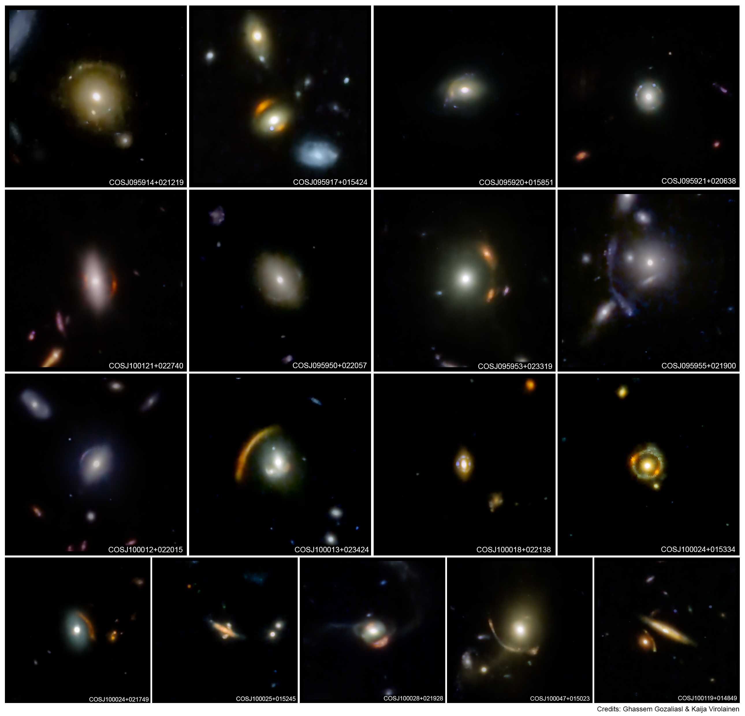
The COWLS sample
Why JAX?
The question is: why port PyAutoLens to JAX for calculating the log-likelihood function?
- Herculens,3 GIGA-Lens4 demonstrated successful adoption of JAX in modeling strong gravitational lensing.
- Performance gains potentially come from:
- Functions implemented with JAX become faster
- Running on accelerators
- Gradient information reduces no. of iterations in fitting
- This project ports the likelihood function, a subset of functionality provided in PyAutoLens, from Numba to JAX
Lesson learnt (programming experience)
Methodology
- Porting
- translate the function to Math
- translate the Math to Numba, using vectorized programming as much as possible to anticipate the programming paradigm in JAX
- translate the Numba function to JAX, where in simple case would just work
- further optimize from there
- Organizing & Testing
- Functions are then kept in 3 different modules,
originalfor the original functions,numbafor those ported in (2),jaxfor those ported in (3) - Metaprogramming is used in setting up unit-test framework (via pytest) to guarantee correctness. pytest-benchmark is used to compare performance differences between these implementations. This feeds back into step (4).
- Functions are then kept in 3 different modules,
What is Numba
- Numba is a jit compiler supporting a subset of Python and NumPy operations, powered by LLVM. While it is possible to target the GPU via CUDA, it requires rewriting the function using different APIs and paradigms, not to mention it is CUDA (i.e. NVidia) only.
What is JAX
- JAX is a jit compiler, tracing compiler by Google, powered by XLA compiler, originated from Google. JAX is designed primarily for machine learning workloads but is suitable for scientific computing as well. It is a tracing compiler removing side-effects of function. I.e. effectively it encourages functional programming paradigm and thinking. It automatically targets multiple hardware architectures including CPU, GPU, TPU, without requiring rewriting.
- I.e. it solves the “two-language problem”, or more accurately, “three-implementation problem”: prototype/API, CPU, GPU.
Numba vs. JAX
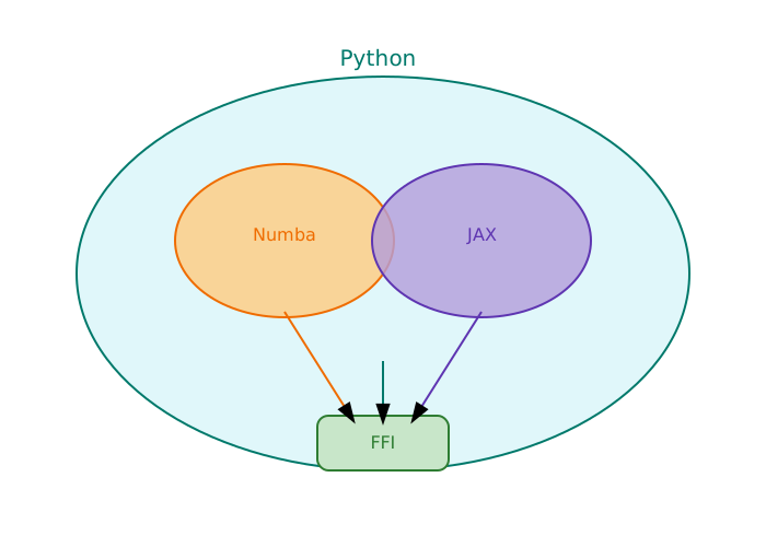
- Numba and JAX are both Domain-Specific Languages (DSLs), with different kinds of fallbacks when complete jit compilation of a function is not possible.
- Better think of it as language + compiler + library.
Numba vs. JAX, side by side
| Numba | JAX |
|---|---|
| C-like mini language | Smaller language (\(\text{JAX} \underset{\sim}{\subset} \text{Numba}\)): restrictions on control flow, mutation, and dynamic shapes |
| Implements a subset of Python+NumPy, with a parallelization model similar to a mini-“OpenMP” | Implements a subset of Python+NumPy+SciPy exposed via duck-typing. |
| NumPy implementations are dropped in replacement but only a subset is implemented. Calling NumPy within jitted function is completely hijacked. Documentation is minimal. | jax.numpy and jax.scipy have similar API comparing to NumPy and SciPy, but has its own documentation. This facilitates deviations in behaviors. |
| Functions “recompile” whenever input type changes. | Functions “recompile” whenever input type and shape changes. |
| No automatic compiling & offloading to accelerator. No autograd/autodiff. | Going through FFI is more costly: memory transfer from and to device, losing autograd/autodiff. |
The documentation point matters more than it looks. Numba’s documentation on its internal workings can be minimal, whereas jax.numpy and jax.scipy have their own comprehensive documentation — which is what makes it practical to deviate from the reference implementation when you need to.
Characteristics of JAX
tracing compiler & recompile per shape change \(\Rightarrow\)
static_argnums@partial(jax.jit, static_argnums=0) def this_recompile_everytime(shape): return jax.numpy.zeros(shape)Compiler Driven Design
- Especially in JAX, partly because of its functional paradigm, framing your problem in JAX idiomatic expressions results in great speed up, sometimes more than you could do otherwise in Numba because of its design (recompile per shape, fusion/fusing compatible operations, etc.), but you’ll hit a wall if you want more low-level optimizations.
- It can also means performance improvements can come for free through compiler improvements, as long as your code is written in JAX idiomatic way.
Easy to port to GPU without setting one up.
JAX vs numba-cuda: The XLA compiler handles device-specific optimization automatically.
JAX nudges you to write correct code, and performance comes as a bonus.
Benchmark analysis
\(\tilde{w}\)—Code: original version
Let’s look at some benchmarks. The function under study here is \(\tilde{w}\), a weight matrix used in the interferometer likelihood:
\[\tilde{W}_{ij} = \sum_{k=1}^K \frac{1}{n_k^2} \cos(2\pi[(g_{i1} - g_{j1})u_{k0} + (g_{i0} - g_{j0})u_{k1}])\]
@numba.jit(nopython=True, nogil=True, parallel=True)
def w_tilde_curvature_interferometer_from(
    noise_map_real: np.ndarray,
    uv_wavelengths: np.ndarray,
    grid_radians_slim: np.ndarray,
) -> np.ndarray:
    w_tilde = np.zeros((grid_radians_slim.shape[0], grid_radians_slim.shape[0]))

    for i in range(w_tilde.shape[0]):
        for j in range(i, w_tilde.shape[1]):
            y_offset = grid_radians_slim[i, 1] - grid_radians_slim[j, 1]
            x_offset = grid_radians_slim[i, 0] - grid_radians_slim[j, 0]

            for vis_1d_index in range(uv_wavelengths.shape[0]):
                w_tilde[i, j] += noise_map_real[vis_1d_index] ** -2.0 * np.cos(
                    2.0
                    * np.pi
                    * (y_offset * uv_wavelengths[vis_1d_index, 0] + x_offset * uv_wavelengths[vis_1d_index, 1])
                )

    for i in range(w_tilde.shape[0]):
        for j in range(i, w_tilde.shape[1]):
            w_tilde[j, i] = w_tilde[i, j]

return w_tilde\(\tilde{w}\)—Code: 1st try
Following the methodology, the first JAX attempt is a direct, fully vectorized transcription of the math:
@jax.jit
def w_tilde_curvature_interferometer_from(
    noise_map_real: np.ndarray[tuple[int], np.float64],
    uv_wavelengths: np.ndarray[tuple[int, int], np.float64],
    grid_radians_slim: np.ndarray[tuple[int, int], np.float64],
) -> np.ndarray[tuple[int, int], np.float64]:
    # (M, M, 1, 2)
    g_ij =  grid_radians_slim.reshape(-1, 1, 1, 2) - grid_radians_slim.reshape(1, -1, 1, 2)
    # (1, 1, K, 2)
    u_k = uv_wavelengths.reshape(1, 1, -1, 2)
    return (
        jnp.cos(
            (2.0 * jnp.pi) *
            # (M, M, K)
            (
                g_ij[:, :, :, 0] * u_k[:, :, :, 1] +
                g_ij[:, :, :, 1] * u_k[:, :, :, 0]
            )
        ) /
        # (1, 1, K)
        jnp.square(noise_map_real).reshape(1, 1, -1)
).sum(2) # sum over k\(\tilde{w}\)—Code: 2nd try
Expanding the cosine of a difference into a product of cosines and sines turns the whole thing into two matrix multiplications:
@jax.jit
def w_tilde_curvature_interferometer_from(
    noise_map_real: np.ndarray[tuple[int], np.float64],
    uv_wavelengths: np.ndarray[tuple[int, int], np.float64],
    grid_radians_slim: np.ndarray[tuple[int, int], np.float64],
) -> np.ndarray[tuple[int, int], np.float64]:
    # A_mk, m<M, k<K
    # assume M > K to put TWO_PI multiplication there
    A = grid_radians_slim @ (TWO_PI * uv_wavelengths)[:, ::-1].T

    noise_map_real_inv = jnp.reciprocal(noise_map_real)
    C = jnp.cos(A) * noise_map_real_inv
    S = jnp.sin(A) * noise_map_real_inv

return C @ C.T + S @ S.T\(\tilde{w}\)—Code: digression in problem sizes
- Number of image pixels
- \(M \sim 70,000 \Rightarrow M^2 \sim 5 \times 10^9, \quad 0 \leq i, j < M\)
- \(N \sim \sqrt{M} \sim 300\)
- Number of visibilities
- \(K \sim 10^7, \quad 0 \leq k < K\)
\((M, M, K, 2)\) of 64-bit array would be \(\sim 700\) PiB!
While \((M, M)\) of 64-bit array would be \(\sim 40\) GiB only.
In other words, the naive vectorized implementation from the 1st try is computationally infeasible — not because the answer is big, but because the intermediate is. The final result is manageable, so the problem is tractable as long as you avoid ever expanding the largest dimension in memory.
\(\tilde{w}\)—Code: final try—Numba
In Numba, the answer is to loop over \(K\) and use prange for a parallel reduction, much like OpenMP:
@numba.jit("f8[:, ::1](f8[::1], f8[:, ::1], f8[:, ::1])", nopython=True, nogil=True, parallel=True)
def w_tilde_curvature_interferometer_from(
    noise_map_real: np.ndarray[tuple[int], np.float64],
    uv_wavelengths: np.ndarray[tuple[int, int], np.float64],
    grid_radians_slim: np.ndarray[tuple[int, int], np.float64],
) -> np.ndarray[tuple[int, int], np.float64]:
    M = grid_radians_slim.shape[0]
    K = uv_wavelengths.shape[0]
    g_2pi = TWO_PI * grid_radians_slim
    δg_2pi = g_2pi.reshape(-1, 1, 2) - g_2pi.reshape(1, -1, 2)

    w = np.zeros((M, M))
    for k in numba.prange(K):
        w += np.cos(δg_2pi[:, :, 1] * uv_wavelengths[k, 0] + δg_2pi[:, :, 0] * uv_wavelengths[k, 1]) * np.reciprocal(
            np.square(noise_map_real[k])
        )
return w\(\tilde{w}\)—Code: final try—JAX
JAX has no prange, and its arrays are immutable, so an in-place reduction is not available. The idiomatic solution is jax.lax.scan, building up the sum iteratively:
@jax.jit
def w_tilde_curvature_interferometer_from(
    noise_map_real: np.ndarray[tuple[int], np.float64],
    uv_wavelengths: np.ndarray[tuple[int, int], np.float64],
    grid_radians_slim: np.ndarray[tuple[int, int], np.float64],
) -> np.ndarray[tuple[int, int], np.float64]:
    M = grid_radians_slim.shape[0]
    g_2pi = TWO_PI * grid_radians_slim
    δg_2pi = g_2pi.reshape(M, 1, 2) - g_2pi.reshape(1, M, 2)
    δg_2pi_y = δg_2pi[:, :, 0]
    δg_2pi_x = δg_2pi[:, :, 1]

    def f_k(
        noise_map_real: float,
        uv_wavelengths: np.ndarray[tuple[int], np.float64],
    ) -> np.ndarray[tuple[int, int], np.float64]:
        return jnp.cos(δg_2pi_x * uv_wavelengths[0] + δg_2pi_y * uv_wavelengths[1]) * jnp.reciprocal(
            jnp.square(noise_map_real)
        )

    def f_scan(
        sum_: np.ndarray[tuple[int, int], np.float64],
        args: tuple[float, np.ndarray[tuple[int], np.float64]],
    ) -> tuple[np.ndarray[tuple[int, int], np.float64], None]:
        noise_map_real, uv_wavelengths = args
        return sum_ + f_k(noise_map_real, uv_wavelengths), None

    res, _ = jax.lax.scan(
        f_scan,
        jnp.zeros((M, M)),
        (
            noise_map_real,
            uv_wavelengths,
        ),
    )
    return res
Match 1: Numba vs JAX with 1 CPU core
| Implementation | s | σ |
|---|---|---|
jax_compact_expanded |
2.5535 (1.0) | 0.0032 |
jax_compact |
2.5543 (1.00) | 0.0050 |
numba_compact |
2.8768 (1.13) | 0.0012 |
numba_compact_expanded |
2.8967 (1.13) | 0.0004 |
original_preload |
11.0392 (4.32) | 0.0010 |
original_preload_expanded |
11.0686 (4.33) | 0.0005 |
jax |
3,368.6229 (>1000.0) | 1.6803 |
original |
3,561.0805 (>1000.0) | 0.2255 |
numba |
3,702.7006 (>1000.0) | 0.7385 |
On a single CPU core, the JAX implementation is slightly faster than the Numba version — about 13%. But look at what changing the underlying algorithm buys you: the compact formulation is a factor of four faster than the best implementation of the original algorithm, and over a thousand times faster than the naive ports of it, all without leaving Numba. Algorithmic improvements can be far more impactful than framework changes.
Match 2: Numba with 128 CPU cores and JAX with CUDA on GPU (A100)
| Implementation | ms | σ |
|---|---|---|
numba_compact |
2.5029 (1.0) | 0.0520 |
numba_compact_expanded |
3.7808 (1.51) | 0.0415 |
jax_compact_expanded |
58.6799 (23.44) | 9.1624 |
jax_compact |
61.5560 (24.59) | 6.8555 |
jax |
143.2451 (57.23) | 0.0749 |
original_preload |
840.0727 (335.63) | 0.1761 |
original_preload_expanded |
842.6588 (336.67) | 0.4933 |
numba |
1,794.1949 (716.83) | 14.9648 |
original |
69,304.2738 (>1000.0) | 13.5543 |
For the original algorithm, JAX on the GPU is significantly faster than Numba on 128 cores — as you’d expect. But for the alternative, compact algorithm, JAX was slower, likely because the problem size was not large enough to saturate the GPU.
Bonus round 1: Numba vs JAX with 1 CPU core (\(F\))
\[F = T^T \tilde{w} T\]
| Implementation | ms | σ |
|---|---|---|
numba_sparse |
8.0733 (1.0) | 0.0501 |
jax |
19.7302 (2.44) | 1.6986 |
jax_sparse |
25.0091 (3.10) | 0.1484 |
jax_BCOO |
48.5340 (6.01) | 0.1571 |
numba_compact_sparse |
49.8400 (6.17) | 0.0794 |
original_preload_direct |
99.2061 (12.29) | 0.3163 |
numba |
125.3019 (15.52) | 0.1143 |
original |
132.4863 (16.41) | 0.1376 |
numba_compact_sparse_direct |
139.9244 (17.33) | 0.1562 |
jax_compact_sparse_BCOO |
379.7214 (47.03) | 1.4144 |
jax_compact_sparse |
380.8865 (47.18) | 2.4322 |
On a single CPU core, the fastest algorithm uses sparse matrix operations in Numba.
Bonus round 2: Numba with 128 CPU cores and JAX with CUDA on GPU (A100) (\(F\))
| Implementation | μs | σ |
|---|---|---|
jax |
260.5957 (1.0) | 29.3714 |
jax_BCOO |
3,078.2068 (11.81) | 35.9463 |
jax_compact_sparse_BCOO |
3,207.3388 (12.31) | 107.0798 |
numba_sparse |
5,548.5175 (21.29) | 64.3711 |
jax_compact_sparse |
7,190.9015 (27.59) | 35.7355 |
numba |
18,187.5003 (69.79) | 5,603.6081 |
original |
18,279.9851 (70.15) | 6,052.1386 |
jax_sparse |
19,786.7200 (75.93) | 42.9344 |
numba_compact_sparse |
32,605.2243 (125.12) | 248.8764 |
numba_compact_sparse_direct |
1,362,329.9249 (>1000.0) | 1,366.9112 |
original_preload_direct |
25,218,633.7856 (>1000.0) | 8,722.4870 |
On the GPU, however, the dense JAX implementation is the fastest by a large margin — and the sparse implementations that won on a single core are now an order of magnitude behind.
Lesson learnt (performance characteristics and expectations)
Takeaway from benchmark analysis
- “Porting Numba to Numba” is faster in many cases
- The only fair fight between Numba and JAX is single CPU core benchmark
- Different algorithms of the same function is faster (even across Numba and JAX) depending on input sizes
- \(\Rightarrow\) keep all implementations \(\rightarrow\) profile \(\rightarrow\) pick best (per science case per system)
Improving the algorithm within Numba can often provide significant speedups without needing to switch frameworks at all.
Limitation of JAX on CPU
JAX for multithreading on the CPU is a rabbit hole. All links below are from GitHub issues. The lack of documentation reflects on the lack of interest in multicore parallelism on the CPU from the primarily machine learning community (JAX from Google, XLA from OpenXLA).
From JAX running in CPU only mode only uses a single core:
This is largely working as intended at the moment. JAX doesn’t parallelize operations across CPU cores unless you use explicit parallelism constructs like pmap. Some JAX operations (e.g., BLAS or LAPACK) operations have their own internal parallelism.
In an HPC setting, you may want to use multiple hierarchies of parallelism on the CPU: SIMD + Multi-threading (e.g. OpenMP) + Multi-processing (e.g. MPI). In this case, you’d want to limit the number of CPU cores for multi-threading, often set via
..._NUM_THREADS. This is very obscure in how to achieve such in JAX:XLA_FLAGS='--xla_cpu_multi_thread_eigen=false intra_op_parallelism_threads=1'was the recommendation. It is now recommended to useNPROC=1to disable multithreading used in Eigen instead. Notice the lack ofJAX_NUM_THREADS\(\Rightarrow\)NPROCmight have side-effects.
export MKL_NUM_THREADS=${NUM_THREADS}
export MKL_DOMAIN_NUM_THREADS="MKL_BLAS=${NUM_THREADS}"
export MKL_DYNAMIC=FALSE

export OMP_NUM_THREADS=${NUM_THREADS}
export OMP_PLACES=threads
export OMP_PROC_BIND=spread
export OMP_DYNAMIC=FALSE

export NUMEXPR_NUM_THREADS=${NUM_THREADS}

export OPENBLAS_NUM_THREADS=${NUM_THREADS}

export NUMBA_NUM_THREADS=${NUM_THREADS}

export NPROC=${NUM_THREADS}
export JAX_NUM_CPU_DEVICES=1
export TF_NUM_INTEROP_THREADS=1
export TF_NUM_INTRAOP_THREADS=${NUM_THREADS}
You may set
JAX_NUM_CPU_DEVICES=${NUM_THREADS}instead, together with sharding to shard your array to different CPU cores. I.e. OpenMP-like parallelism cannot be achieved. Also,jax.device_putrequires your array length is divisible byJAX_NUM_CPU_DEVICES.- Preliminary tests are not promising.
Lessons learnt from Numba vs. JAX
- Does it solve the “3-implementation problem”?
- prototype:
original - multithreading on the CPU:
numba - running on accelerator:
jax
- prototype:
- Even if we compare JAX and Numba on equal footing (a single CPU core): sometimes it is faster with JAX (e.g. compiler optimization w.r.t. shape, fusion, etc.) but sometimes it is faster with Numba as JAX language is more restrictive and hence Numba allows expression of more efficient algorithms (recall \(\text{JAX} \underset{\sim}{\subset} \text{Numba}\))
- Therefore I think it is advantageous to keep both Numba and JAX implementation. See more from Should Numba be dropped completely? | AutoJAX Doc
Miscellaneous notes
- Decouple algorithmic development (“library code”) and Python API, e.g. allow end users to choose backends between Numba and JAX. This also facilitate future porting to, say, Julia.
- Open problems: Delaunay/Voronoi mesh is going to be difficult to implement as JAX’s programming model dislikes dynamic shapes.
- Don’t wrestle with the language, especially for DSLs
Conclusions
- Bayesian inference in cosmology is fun!
- JAX is a fun(tional) language to work with
- ✓ very easy to deploy to accelerators
- ✗ more restrictive in language features
- ✗ poor on CPU multithreading
It is a powerful language with a pure functional paradigm that makes it easy to achieve great speedups and deploy on GPUs. But it is not a silver bullet for all HPC use cases, particularly those relying heavily on multi-core CPU parallelism. Thank you.
Team, Links, & References
- PyAutoLens Team
- James W. Nightingale
- Richard G. Hayes
- Aristeidis Amvrosiadis
- Coleman Krawczyk
- Gokmen Kilic
- …
- Link of this project: https://ickc.github.io/python-autojax/. This is a standalone framework to compare different implementations of functions. Functions are being upstreamed to PyAutoLens.
References
Footnotes
“Scanning for Dark Matter Subhaloes in Hubble Space Telescope Imaging of 54 Strong Lenses,” Monthly Notices of the Royal Astronomical Society 527, no. 4 (2023): 10480–506, https://doi.org/10.1093/mnras/stad3694.↩︎
Guillaume Mahler et al., “The COSMOS-Web Lens Survey (COWLS) II: Depth, Resolution, and NIR Coverage from JWST Reveal 17 Spectacular Lenses,” arXiv:2503.08782, preprint, arXiv, March 11, 2025, https://doi.org/10.48550/arXiv.2503.08782.↩︎
A. Galan et al., “Using Wavelets to Capture Deviations from Smoothness in Galaxy-Scale Strong Lenses,” Astronomy & Astrophysics 668 (December 2022): A155, https://doi.org/10.1051/0004-6361/202244464.↩︎
A. Gu et al., “GIGA-Lens: Fast Bayesian Inference for Strong Gravitational Lens Modeling,” The Astrophysical Journal 935, no. 1 (2022): 49, https://doi.org/10.3847/1538-4357/ac6de4.↩︎