JIT compilers for scientific computing in Python: Numba vs. JAX
A Case Study Evaluating Gravitational Lensing Likelihood
Accelerating scientific Python with JITs. We share our journey migrating a gravitational lensing likelihood calculation from Numba to JAX. Learn about performance gains, automatic differentiation benefits, and practical lessons for high-performance scientific computing in Python.
Python is widely used in scientific research, but pure Python can sometimes be too slow for computationally intensive tasks. Just-In-Time (JIT) compilers are essential tools for boosting performance, allowing Python code to run closer to native speeds. While libraries like Numba have long been popular for accelerating numerical Python functions, JAX offers a new paradigm, combining JIT compilation with powerful features like automatic differentiation (auto-diff) and execution across different hardware (CPUs, GPUs, TPUs).
This talk will take you on a journey through our experience optimizing a critical component of an astrophysics analysis pipeline: the calculation of the likelihood function for gravitational lensing models, used with data from the James Webb Space Telescope. We initially used Numba to accelerate this calculation, but the need for performance portability across hardwares, and the potential speed up from gradient computation for model fitting led us to explore JAX’s unique capabilities.
This session will walk through the practical steps, challenges, and insights gained from migrating this complex scientific code from its existing Numba implementation to a JAX-based one.
You will learn:
- Why leveraging performance tools like JITs is crucial for cutting-edge scientific analysis in Python.
- The practical considerations when migrating existing numerical code from Numba to JAX, including syntax changes and managing state.
- How JAX’s auto-differentiation simplifies gradient calculations essential for scientific optimization and sampling tasks.
- The significant performance improvements achieved in our specific gravitational lensing case study by using JAX’s compiled functions.
- Broader lessons learned about structuring scientific Python projects to effectively use modern JIT compilers and harness capabilities like auto-diff.
We’ll conclude by comparing Numba and JAX in benchmark performance, developer ergonomics, and tradeoffs between the two, providing you with practical guidance for choosing the right tool for your scientific computing needs.
This case study offers a concrete example of how evolving Python libraries are enabling researchers to perform complex, high-performance computations directly within the Python ecosystem. Join us to see how tools like JAX are empowering scientific discoveries, one optimised function at a time.
This talk is suitable for intermediate Python programmers familiar with NumPy.
Below is a companion article to the PyCon UK 2025 talk on porting a gravitational lensing likelihood from Numba to JAX for JWST analysis. The slides and this article are generated from a single source, so everything that was on screen is here, together with what was said around it.
Today I’m going to talk about JIT compilers for scientific computing in Python — Numba versus JAX — through a case study on evaluating a gravitational lensing likelihood.
Context: Why Python in HPC?
Why do I use Python in HPC?
- Cosmologist
- PhD: CMB Data Analysis
- processing \(\sim O(10\text{ TiB}) \sim O(\text{PiB})\) of data for cosmological inference
- using scientific softwares in Python
- running on NERSC (a top 10 HPC system)
Let me start with why I use it.
I am a cosmologist. I did my PhD in the UC Berkeley Physics department on the topic of the Cosmic Microwave Background (CMB) radiation — the relic radiation that is everywhere, so that every time you look at the sky you are looking at it, you just don’t know it. During my research I used the NERSC HPC facility in the US, a top 10 supercomputing system, to perform CMB data analysis. HPC stands for High Performance Computing, also known as supercomputing.
Briefly speaking, as we cannot do an experiment cosmologically, we instead observe a huge amount of data and use statistical methods such as Bayesian inference to deduce information about our universe, such as deducing the dark matter composition, or finding evidence of inflation during the Big Bang. My main interest in Python is therefore primarily its application to scientific computing on HPC.
Questions: which language can you use to write applications for HPC?
Languages that has demonstrated to scale to state-of-the-art, full system supercomputer
- Fortran
- C/C++
- Python
- Julia
matlabrust
This was a question to the room, so treat it as one here too. By “can you use”, I mean a language that has demonstrated it scales to a state-of-the-art, full-system supercomputer — not merely a language you can invoke on one, the way you would invoke bash.
The room got Fortran and C/C++ immediately. The next answer is Python, and you might call that cheating a little bit, because many of the codes you call from Python to run on an HPC system were written in Fortran or C and are simply exposed as a module. It is still very useful as the glue that holds everything together. Julia belongs on the list as well. MATLAB and Rust do not — not because they are bad languages, but because they have not yet demonstrated that they scale to a full system.
Questions: Why Python in HPC? What is its superpower in supercomputing?
- Because it is where the community is.
- Because we are the people who don’t care what language our algorithm is implemented in.
- C
- C++
- Fortran
- Julia
- Rust
- …
The opening keynote resonates with me a lot. Python has superpowers. I recommend people watching that to see the history and the bigger picture. Here, I am more narrowly focused to tell you why, at this particular moment, Python is the language of choice to write and run scientific applications on supercomputers.
The room offered embarrassingly parallel workloads, and developer efficiency. Both are true — and even when the problem is not embarrassingly parallel you can still drive it from Python. But my own answer is this.
First of all, it is where the community is. NumPy, SciPy, Astropy, you name it. I am not claiming to explain how it got here, or whether it will still be the case in the future; only that at this moment, this is where the community is.
Secondly — and I don’t know whether this is a blasphemy — it is because we are the people who don’t care what language our algorithm is implemented in. CPython itself is written in C. C++ is exposed as a Python module through pybind11. Many SciPy functions are Fortran underneath. Write something in Julia, or in Rust, and you can still expose it with a Python interface.
In other words, Python is the glue. If we look back to the list of languages that has demonstrate they can scale to the state-of-the-art supercomputer at a given era, there is not a lot on the list, and Python is one of them. You might call that cheating, because in this case Python is mostly just calling C modules or libraries written in Fortran. But we don’t care. Python is the glue that successfully composed very complicated scientific workflow together.
Context: Why JIT?
Short introduction on aot/jit compilations & interpreter
- interpreters
- CPython
- bash
- compilers
- AOT
gccfrom GNU compilers,clangfrom LLVM compilers- CPython is AOT compiled by these compilers!
- traditionally excels at HPC: C/C++, Fortran
- JIT
pypy- Julia
- Javascript has a JIT
- AOT
So, why JIT? To answer that I need to give two short introductions first.
Back to the languages, focusing on the aspect of how source code eventually runs, it falls into two categories, compilers and interpreters. And within compilers, there are also ahead-of-time (AOT) compilation and just-in-time (JIT) compilation.
Here we will name a few examples. The reference Python implementation, CPython, is an interpreter, which is AOT compiled by C compilers such as gcc and clang. Bash is another commonly used interpreted language, and I would say that in the HPC space, Python is increasingly taking over what bash used to do. AOT compilation is what traditionally excels at HPC: C, C++, Fortran.
Another well known Python implementation pypy is a jit compiler — supposedly any valid Python program can run under it. Julia and JavaScript have JITs too.
Short introduction on the landscape of acceleration framework of numeric code in Python
- AOT
- C with CPython API
- e.g. Numpy, which is a framework in itself
- Cython: superset of the Python language, compiled to C modules, handle CPython API and Python interface automatically
- pybind11: C++ 11+, handle CPython API and Python interface semi-automatically
- C with CPython API
- JIT
pypy: general purpose Python implementation (any valid Python should runs)- CPython 3.13+ experimental JIT: only a subset of Python code will be jit compiled (and is not clear on when and where), not focused on numerical
- Numba, JAX: DSL, jit-compile a subset of Python, focused on numerical
The second introduction is how you accelerate a piece of Python code when you need to.
I hope we all agree the CPython interpreter is slow, right? To accelerate applications running in CPython, there are multiple frameworks to do it. The traditional model is C modules: write your performance critical part of the code in C and use the CPython API to expose a Python interface to the users. A prominent example of that is numpy, which defines an interface often used in high performance numerical operations, and is architected in C with a pythontic interface. This is still one of the fastest and pythonic way to write numerical code in Python without introducing further compliation to the users. Other examples on AOT are cython and C++ with pybind11, which I won’t go into details.
Turning our attention to the spotlight of the day: JIT. pypy is a general purpose Python jit compiled runtime for a long time. There is also an experimental JIT compiler in CPython 3.13+, which would jit compiled a subset of hot code: anything valid still runs, but only some of it is actually compiled, and it is not aimed at numerics.
The remaining JIT compilers are the one we are focusing on today. Numba and JAX can both be regarded as Domain Specfic Languages that will jit compiled a subset of the Python language, focused on numerical compuations.
Why jit: solving the 2 language problem
To replace this single function from Numba to C++ with pybind11,
@numba.jit(parallel=True)
def _fma(out, weights, *arrays):
    for weight, array in zip(weights, arrays):
out += weight * array14 files changed
+230 -36 lines changed… and 30% faster!
Python gives you velocity: rapid prototyping science code is a path dependent evolution
Numba jit gives you speed (SIMD + multi-threading): C++ with SIMD and OpenMP multi-threading is only 30% faster in this case. The single
@jitdecorator gives you 3 times speed up comparing to pure Numpy implementation.JIT sometimes has advantage over AOT because it can see the data
JIT obviously has overhead, but if you are processing “big data”, that amount of time usually is much shorter than it takes to run the calculation itself.
My headline answer to “why JIT” is that it solves the two-language problem: you no longer need two different languages to implement very high performance code.
To briefly give an idea why JIT may be useful, we can look at this function as an example. If you are familiar with Numba enough, as soon as you write down this simple function with Numpy, adding the jit decorator there is a no-brainer. You would be able to immediately predict that it will be faster — three times faster than the pure NumPy version, in this case — and that memory allocation is simpler, and hence lesser memory pressure and lesser chance of getting killed by out-of-memory (OOM) error.
However, when I ported this to C++ with pybind11, 14 files are changed, 230 lines are added. If you look into the commit change, for sure a lot of them are boilerplates. But that is exactly the point. It went from using Numba as a 10s decision to being 30% faster after a ton of work. One single line gave three times; all of that work gave 30%.
This sort of things happens all the time when writing science code. How your program eventually got there is often not obvious in the beginning. It involves repid prototyping and sometimes solving complicated mathematical or algorithmic problems. Having a DSL within Python that can be jitted is a superpower Python given us to move fast and run fast at the same time.
Concrete example of Numba vs. JAX
\(\tilde{w}\)
\[\tilde{w}_{ij} = \sum_{k=1}^K \frac{1}{n_k^2} \cos \left( 2 \pi \left[ \left(\vec{g}_i - \vec{g}_j \right) \cdot \vec{u}_k \right] \right) ,\quad 1 \leq i, j \leq M\]
Now it all makes sense, kind of. Let us do an actual example to see how JIT works.
I call this a slow track. It is a live demo without being live. I hope it will gives you a feel of the languages and gain intuitions yourself. Later on, we will have a fast track and you just have to believe the high level summaries I am going to give you.
Let’s stare at this equation and see how you would implement it.
Numpy
As usual in Numpy, we vectorize everything:
import numpy as np


def w_mm_np(
    n_k: np.ndarray[tuple[int], np.float64],
    u_k_vec: np.ndarray[tuple[int, int], np.float64],
    g_m_vec: np.ndarray[tuple[int, int], np.float64],
) -> np.ndarray[tuple[int, int], np.float64]:
    # (M, M, 1, 2)
    δg_mm1_vec =  g_m_vec.reshape(-1, 1, 1, 2) - g_m_vec.reshape(1, -1, 1, 2)
    # (1, 1, K, 2)
    u_11k_vec = u_k_vec.reshape(1, 1, -1, 2)
    return (
        np.cos(
            (2.0 * np.pi) *
            # (M, M, K)
            (
                δg_mm1_vec[:, :, :, 0] * u_11k_vec[:, :, :, 1] +
                δg_mm1_vec[:, :, :, 1] * u_11k_vec[:, :, :, 0]
            )
        ) /
        # (1, 1, K)
        np.square(n_k).reshape(1, 1, -1)
    ).sum(2)  # sum over k
898 ms ± 9.62 ms per loop (mean ± std. dev. of 7 runs, 1 loop each)The function is not really very long — it is almost a one-liner. I have just given it a lot of whitespace to make it clearer what is happening, but it is only implementing the math as it is written. And it is reasonably fast.
Ignore the tiny little details there where the order of the dimensions in \(\vec{g}\) and \(\vec{u}\) are opposite to each other.
Numba
How would you implement it in Numba? Just add the jit decorator:
import numba


@numba.jit("f8[:, ::1](f8[::1], f8[:, ::1], f8[:, ::1])", nopython=True, nogil=True, parallel=True)
def w_mm_numba(
    ...
522 ms ± 9.01 ms per loop (mean ± std. dev. of 7 runs, 1 loop each)Mine looks a little complicated, but the part that really makes the difference is parallel=True. It is a very simple decorator to add, and you can immediately see that it is faster.
JAX
How would you implement it in JAX? By add the jit decorator, and replacing numpy with jax.numpy:
import jax
import jax.numpy as jnp

@jax.jit
def w_mm_jax(
    n_k: np.ndarray[tuple[int], np.float64],
    u_k_vec: np.ndarray[tuple[int, int], np.float64],
    g_m_vec: np.ndarray[tuple[int, int], np.float64],
) -> np.ndarray[tuple[int, int], np.float64]:
    # (M, M, 1, 2)
    δg_mm1_vec =  g_m_vec.reshape(-1, 1, 1, 2) - g_m_vec.reshape(1, -1, 1, 2)
    # (1, 1, K, 2)
    u_11k_vec = u_k_vec.reshape(1, 1, -1, 2)
    return (
        jnp.cos(
            (2.0 * jnp.pi) *
            # (M, M, K)
            (
                δg_mm1_vec[:, :, :, 0] * u_11k_vec[:, :, :, 1] +
                δg_mm1_vec[:, :, :, 1] * u_11k_vec[:, :, :, 0]
            )
        ) /
        # (1, 1, K)
        jnp.square(n_k).reshape(1, 1, -1)
    ).sum(2)  # sum over k
144 ms ± 1.53 ms per loop (mean ± std. dev. of 7 runs, 10 loops each)Can you guess? Just change the decorator — plus one more thing. Plain NumPy does not work inside a JAX-jitted function, but JAX ships its own module, jax.numpy, which is almost a drop-in replacement: wherever you had np, you use jnp, conventionally imported under that name, and it works.
You would notice the speed up from Numpy to Numba to JAX, in this order, which is often the case. There is a general trend of progress here: you start with something in NumPy, you implement it in Numba and it is faster, and then in JAX — where it is not even a reimplementation, just a change in how it is compiled — and it is faster still. That is the general trend, though I am not saying this is always the case.
Ok, case closed, right?
Hold on, not so fast. Does anyone spot any potential problem with this implementation?
Case closed?
All three implementations are the same in this respect, so here is a hint: go back to the NumPy listing and look at the comment marking (M, M, K). What it means is that an array of that shape is materialized at that point in the expression.
Digression in problem sizes
\[\tilde{w}_{ij} = \sum_{k=1}^K \frac{1}{n_k^2} \cos \left( 2 \pi \left[ \left(\vec{g}_i - \vec{g}_j \right) \cdot \vec{u}_k \right] \right) ,\quad 1 \leq i, j \leq M\]
- Number of image pixels
- \(M \sim 70,000 \Rightarrow M^2 \sim 5 \times 10^9, \quad 0 \leq i, j < M\)
- Number of visibilities
- \(K \sim 10^7, \quad 0 \leq k < K\)
\((M, M, K, 2)\) of 64-bit array would be \(\sim 700\) PiB!
While \((M, M)\) of 64-bit array would be \(\sim 40\) GiB only.
To put that into perspective, whole system aggregated memory of NERSC is \(\sim 2\text{ PiB}\).
I haven’t told you yet how large the problem is. \(\tilde{w}_{ij}\) is an \(M \times M\) matrix, where \(M\) is the number of image pixels and can be as large as 70,000. \(K\) is the number of so-called visibilities, and can be as large as \(10^7\). So if you work out the size of the array being created at that intermediate step, it is on the order of hundreds of PiB. There is simply no computer that will fit that in memory.
The answer itself is fine — an \((M, M)\) array of 64-bit floats is about 40 GiB. The problem is not the answer, it is the intermediate.
Numpy—low memory version
- avoid expanding \(K\)
The solution is simple, we do not want to expand the \(K\)-dimension fully in memory. We want to evaluate that lazily and accumulate it over \(k\).
How would you do that in NumPy? You can always write a Python loop over \(k\) — but would that be efficient? Probably not. There is no efficient solution in numpy however without using Python loops. I think there isn’t one; I can’t prove it. Let me know if you know a way.
Numba—low memory version
@numba.jit("f8[:, ::1](f8[::1], f8[:, ::1], f8[:, ::1])", nopython=True, nogil=True, parallel=True)
def w_mm_numba_iterative(
    n_k: np.ndarray[tuple[int], np.float64],
    u_k_vec: np.ndarray[tuple[int, int], np.float64],
    g_m_vec: np.ndarray[tuple[int, int], np.float64],
) -> np.ndarray[tuple[int, int], np.float64]:
    M = g_m_vec.shape[0]
    K = u_k_vec.shape[0]
    δg_mm_vec = g_m_vec.reshape(-1, 1, 2) - g_m_vec.reshape(1, -1, 2)

    w_mm = np.zeros((M, M))
    for k in numba.prange(K):
        w_mm += np.cos((2.0 * np.pi) * (δg_mm_vec[:, :, 1] * u_k_vec[k, 0] + δg_mm_vec[:, :, 0] * u_k_vec[k, 1])) / np.square(n_k[k])
    return w_mm
55 ms ± 1.59 ms per loop (mean ± std. dev. of 7 runs, 10 loops each)In Numba, however, we can have efficient loops, we can even do it in parallel. This function looks very similar to the version before: that one line is computing the same equation for a fixed value of \(k\), you loop over \(k\), and you do an in-place reduced sum. That is all. It will handles the reduced sum there in parallel correctly for you. It actually maps very nicely to C with SIMD and OpenMP parallel-for there. In fact, OpenMP is one of the threading layer backend in Numba.
A large part of why it is this fast is numba.prange, which parallelizes the loop.
JAX—low memory version
@jax.jit
def w_mm_jax_iterative(
    n_k: np.ndarray[tuple[int], np.float64],
    u_k_vec: np.ndarray[tuple[int, int], np.float64],
    g_m_vec: np.ndarray[tuple[int, int], np.float64],
) -> np.ndarray[tuple[int, int], np.float64]:
    M = g_m_vec.shape[0]
    δg_mm_vec = g_m_vec.reshape(M, 1, 2) - g_m_vec.reshape(1, M, 2)
    δg_mm_y = δg_mm_vec[:, :, 0]
    δg_mm_x = δg_mm_vec[:, :, 1]

    def _w_mm_k(
        n: float,
        u_vec: np.ndarray[tuple[int], np.float64],
    ) -> np.ndarray[tuple[int, int], np.float64]:
        return jnp.cos((2.0 * jnp.pi) * (δg_mm_x * u_vec[0] + δg_mm_y * u_vec[1])) / (n * n)

    def _accumulate_w_mm(
        sum_: np.ndarray[tuple[int, int], np.float64],
        args: tuple[float, np.ndarray[tuple[int], np.float64]],
    ) -> tuple[np.ndarray[tuple[int, int], np.float64], None]:
        n, u_vec = args
        return sum_ + _w_mm_k(n, u_vec), None

    res, _ = jax.lax.scan(
        _accumulate_w_mm,
        jnp.zeros((M, M)),
        (
            n_k,
            u_k_vec,
        ),
    )
    return res
86.6 ms ± 102 μs per loop (mean ± std. dev. of 7 runs, 10 loops each)This means we can does the same in JAX, right? Wrong. It is very tempting to just swap the decorator — that is the whole promise of a decorator, that you put it there and it works — but here it won’t.
This is where one of the core design of JAX matters. JAX is essentially designed with pure functional programming paradigm in mind. It enforces immutable data, where the in-place reduced sum there is prohibited. JAX dislikes anything that mutates your state.
It does not mean it does not have semantics for looping. To express exactly the same logic, you refactor it in a certain way: a kernel function evaluating the same equation for one particular value of \(k\), and then a way to tell the program to iterate over all \(k\) and sum them up. Here, I choose scan, one of the idiomatic JAX interfaces for that, and itself a functional programming construct. What it does basically is to focus on each term for a dixed \(k\), and then accumulate the sum over different values of \(k\). If you believe me, this represents almost exactly the same thing as the Numba version, in the JAX-idiomatic way.
See python-autojax/experiments/reduced_sum at main · ickc/python-autojax for more details on how this can be expressed in JAX.
Numba vs. JAX on paper
What is Numba / JAX
- Numba
- jit compiler powered by LLVM compiler
- CPU only
numba.cudais an entirely different interface
- JAX
- tracing, jit compiler powered by XLA compiler
- designed for machine learning workflow
- no side effects \(\rightarrow\) functional paradiagm
- targets CPU, GPU (NVidia, AMD, Intel, Apple), TPU simultaneously
- solving 2 language problem
- solving “3 implementations problem”
- Better think of them as language + compiler + library
This section is the fast track, and it is a bit denser than the rest. On the day I was short on time and skipped some of it; the article does not have to.
Now that we have seen some examples on how jit works, we will introduce them once more in details.
Numba is a jit compiler supporting a subset of Python and NumPy operations, powered by LLVM. While it is possible to target the GPU via CUDA, it requires rewriting the function using different APIs and paradigms, not to mention it is CUDA (i.e. NVidia) only.
JAX is a jit compiler, tracing compiler by Google, powered by XLA compiler, originated from Google. XLA stands for Accelerated Linear Algebra, which already tells you where its focus lies. JAX is designed primarily for machine learning workloads but is suitable for scientific computing as well, because the two have a lot in common. It is a tracing compiler removing side-effects of function. I.e. effectively it encourages functional programming paradigm and thinking. It automatically targets multiple hardware architectures including CPU, GPU, TPU, without requiring rewriting. I.e. it solves the “two-language problem”, or more accurately, “three-implementation problem”: prototype/API, CPU, GPU.
This is where JAX shines over other solutions to develop for the GPU. In principle, one single implementation is all you need. You do not need to optimize a function for the CPU, optimize another for the GPU.
One more tip for thinking about either of them: it is better to regard the thing named “Numba” or “JAX” as a language, a compiler, and a library all at once. A domain-specific language, because not everything can be jit-compiled; a compiler that does the compiling; and a set of libraries that come along with it. The comparison below is organized along those three lines.
Numba vs. JAX
| Numba | JAX |
|---|---|
| C-like mini language | Smaller language (\(\text{JAX} \underset{\sim}{\subset} \text{Numba}\)): restrictions on control flow, mutation, and dynamic shapes |
| Implements a subset of Python+NumPy, with a parallelization model similar to a mini-“OpenMP” | Implements a subset of Python+NumPy+SciPy exposed via duck-typing. |
| NumPy implementations are dropped in replacement but only a subset is implemented. Calling NumPy within jitted function is completely hijacked. Documentation is minimal. | jax.numpy and jax.scipy have similar API comparing to NumPy and SciPy, but has its own documentation. This facilitates deviations in behaviors. |
| Functions “recompile” whenever input type changes. | Functions “recompile” whenever input type and shape changes. |
| No automatic compiling & offloading to accelerator. No autograd/autodiff. | Going through FFI is more costly: memory transfer from and to device, losing autograd/autodiff. |
As a language, Numba is more like a C-like mini language: mostly anything you can express in C can be expressed in Numba. JAX is a smaller language still — more restrictions on control flow, on mutation, and on dynamic shapes; you basically cannot do any of those.
As a library, Numba implements a subset of Python and NumPy with a parallelization model of its own. NumPy in Numba is a drop-in replacement, but only a subset of those operations is implemented, and whenever NumPy is called within a Numba jit-compiled function, it is completely hijacked: it is not really calling NumPy, Numba takes over and does its own thing. JAX, on the other hand, implements a subset of Python, NumPy and SciPy, so it is the larger library, and it lives in its own namespaces, jax.numpy and jax.scipy. The APIs are similar to NumPy and SciPy — most of them are the same — but they have their own documentation, and that documentation is precisely what makes it practical for JAX to deviate in behavior where its own restrictions, such as the functional paradigm we mentioned, require it.
Characteristics of JAX
tracing compiler & recompile per shape change \(\Rightarrow\)
static_argnums@partial(jax.jit, static_argnums=0) def this_recompile_everytime(shape): return jax.numpy.zeros(shape)Compiler Driven Design
- Especially in JAX, partly because of its functional paradigm, framing your problem in JAX idiomatic expressions results in great speed up, sometimes more than you could do otherwise in Numba because of its design (recompile per shape, fusion/fusing compatible operations, etc.), but you’ll hit a wall if you want more low-level optimizations.
- It can also means performance improvements can come for free through compiler improvements, as long as your code is written in JAX idiomatic way.
Easy to port to GPU without setting one up.
JAX vs numba-cuda: The XLA compiler handles device-specific optimization automatically.
As a functional language, JAX nudges you to write correct code, and performance comes as a bonus.
A few characteristics are worth internalizing. Because JAX is a tracing compiler that recompiles per shape change, anything that is genuinely a compile-time constant — a shape, for instance — has to be marked as such with static_argnums, or you recompile on every call.
More broadly, I think of this as compiler driven design. The upside is that performance improvements can arrive for free through compiler improvements, so long as your code is written the idiomatic way; the downside is the wall you hit when you want low-level control. It is a trade you make knowingly.
When not to JIT in Python?
- Don’t wrestle with languages, choose something else
- AOT: C++ + pybind11
- JIT: Julia
If you find yourself wrestling against the language, deviating from idioms and best practices, time to choose something else!
These are DSLs. They are small on purpose, and the moment you are fighting the smallness rather than using it, the honest move is to step outside: C++ with pybind11 if you want ahead-of-time compilation, Julia if you want a JIT.
Numba vs. JAX: case study of PyAutoLens
Benchmark: Numba vs JAX with 1 CPU core
\[\tilde{w}_{ij} = \sum_{k=1}^K \frac{1}{n_k^2} \cos \left( 2 \pi \left[ \left(\vec{g}_i - \vec{g}_j \right) \cdot \vec{u}_k \right] \right) ,\quad 1 \leq i, j \leq M\]
| Implementation | s | σ |
|---|---|---|
jax_compact |
2.5543 (1.00) | 0.0050 |
numba_compact |
2.8768 (1.13) | 0.0012 |
jax |
3,368.6229 (>1000.0) | 1.6803 |
numba |
3,702.7006 (>1000.0) | 0.7385 |
Everything so far has been leading to why I actually did this work. The case study is PyAutoLens: a project with a very complicated science codebase, originally implemented in Numba, and I am part of the effort that brought the whole thing to JAX.
We previously have seen different implementations of \(\tilde{w}\) and some informal benchmarks.
Here we are seeing the benchmark generated using the actual library I wrote.
The numba and jax in this table corresponds to the low memory implementation we’ve shown previously. We see that given 1 single CPU core, the JAX version is slightly faster than the Numba version.
But more importantly, we see that there is a _compact version that I have not shown before. This is 3 orders of magnitude faster. This is done by taking advantage of the fact that δg there has a lot of repeatitive values. The algorithm that I shown to you is \(O(M^2)\) while the compact version is \(O(M)\).
This also illustrates that sometimes you can focus on low level optimization and have 30% speed up. Or you could spend your time instead on the mathematics behind it and find a better algorithm that can achieves unlimited amount of speed up.
Benchmark: Numba with 128 CPU cores and JAX with CUDA on GPU (A100)
| Implementation | ms | σ |
|---|---|---|
numba_compact |
2.5029 (1.0) | 0.0520 |
jax_compact |
61.5560 (24.59) | 6.8555 |
jax |
143.2451 (57.23) | 0.0749 |
numba |
1,794.1949 (716.83) | 14.9648 |
Now how about the million dollar question, how would JAX perform on the GPU? Since the Numba implementation cannot run on the GPU, let us give it a boost to have some resembance of fair fight, 128 CPU cores, vs. JAX on the NVidia A100.
(Notice the slight change of problem size here.)
What we see is the Numba version scales almost perfectly with 128 CPU cores. The JAX implementation is however another order of magnitude faster.
What happens for the compact case though? I think it is because they are so efficient so that the problem size is not big enough to “warm up” the GPU. But note that it is not a fair fight anyway, as we can talking about comparing benchmark from different hardware.
Bonus round 1: Numba vs JAX with 1 CPU core (\(F\))
\[F = T^T \tilde{w} T\]
| Implementation | ms | σ |
|---|---|---|
numba_sparse |
8.0733 (1.0) | 0.0501 |
jax |
19.7302 (2.44) | 1.6986 |
jax_sparse |
25.0091 (3.10) | 0.1484 |
jax_BCOO |
48.5340 (6.01) | 0.1571 |
numba_compact_sparse |
49.8400 (6.17) | 0.0794 |
original_preload_direct |
99.2061 (12.29) | 0.3163 |
numba |
125.3019 (15.52) | 0.1143 |
original |
132.4863 (16.41) | 0.1376 |
numba_compact_sparse_direct |
139.9244 (17.33) | 0.1562 |
jax_compact_sparse_BCOO |
379.7214 (47.03) | 1.4144 |
jax_compact_sparse |
380.8865 (47.18) | 2.4322 |
Just to give you one more benchmark to look at, here is another complicated example I have done in the project. You are already familar with \(\tilde{w}\), where as \(T\) here can be a sparse matrix.
While I am not going into details here, but there is a bunch of combinatorics here. Should we calculate \(\tilde{w}\) directly, or go through the compact version? Should we use the sparse structure of matrix \(T\), or expand that in memory first?
My claim is that this depends on the size of input data, and which is the fastest to choose from depends on your data which can be informed by benchmark like this.
Bonus round 2: Numba with 128 CPU cores and JAX with CUDA on GPU (A100) (\(F\))
| Implementation | μs | σ |
|---|---|---|
jax |
260.5957 (1.0) | 29.3714 |
jax_BCOO |
3,078.2068 (11.81) | 35.9463 |
jax_compact_sparse_BCOO |
3,207.3388 (12.31) | 107.0798 |
numba_sparse |
5,548.5175 (21.29) | 64.3711 |
jax_compact_sparse |
7,190.9015 (27.59) | 35.7355 |
numba |
18,187.5003 (69.79) | 5,603.6081 |
original |
18,279.9851 (70.15) | 6,052.1386 |
jax_sparse |
19,786.7200 (75.93) | 42.9344 |
numba_compact_sparse |
32,605.2243 (125.12) | 248.8764 |
numba_compact_sparse_direct |
1,362,329.9249 (>1000.0) | 1,366.9112 |
original_preload_direct |
25,218,633.7856 (>1000.0) | 8,722.4870 |
Looking at how JAX runs on the GPU, surprisingly the simplest implementation is fastest. Again I suspect there is not enough data for those faster algorithm to flex its muscle.
Flow chart
If either Numba or JAX have enough feature to acommplish what you need, performance-wise, here’s a flowchart:

If you have to pick between the two based on my experience, this is where each one lands. It is not the only thing you can do, but it captures the shape of the decision.
There is one situation where Numba is genuinely better than JAX: if you only target the CPU, you know you have a lot of CPU cores available, and your problem is not linear-algebra heavy. In that corner Numba wins. Most of the time, though, JAX is quite good.
What JIT has enabled in scientific computing?
Context: Maximal Likelihood Estimation (MLE)
- \(\tilde{w}, T, F\), etc. are part of a likelihood function
- Aim: seek the input parameters corresponding to maximum likelihood
- \(\Rightarrow\) peak finding
- Gradient information is going to be useful here.
- JAX another secret weapon: autodiff / autograd (
jax.grad)- compilers can transform code
- transform function to find its gradient automatically
Now, let’s see what JIT has enabled our science.
I am not going to give these graphs a justice. But, I am going to have a crash course here and jump to conclusion. The \(\tilde{w}, T, F\), etc. you have seen before is part of a calculation known as the likelihood function. The \(\tilde{w}\) is a big part of turning the observed data into a likelihood function. Now you can make predictions from models given some parameters. and the likelihood function is going to tell you how likely those parameters are. Using different kinds of samplers, which all involve running the likelihood functions repeatedly, often with \(O(100,000)\) of iterations. And the parameters that corresponds to the maximum likelihood is simply called the maximal likelihood estmator (MLE).
This is basically how we do inverse problem statistically. And obviously it is some kind of maximization problem.
There is one thing about JAX I have not told you yet, and it belongs here. If you are looking for a peak, gradient information is obviously useful: the gradient already tells you roughly where the peak is, pointing you in the right direction. And now that things are jit-compiled, consider what compilers actually do — they transform code. You have code written one way and it is transformed into another. So why not leverage that to transform your function into its gradient as well? That is exactly what automatic differentiation, jax.grad, does, and in a science case like this it is a real advantage.
MLE in action
- 25 free parameters
- Lens Light (11): Sersic + Exponential
- Lens Mass (7): SIE + Shear
- Source Light (7): Sersic
PyAutoLens (via PyAutoFit) supports Nested sampling (Dynesty), MCMC (emcee), particle swarm optimization (PySwarms)
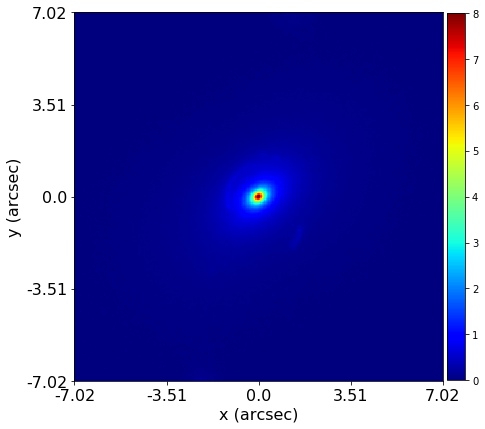
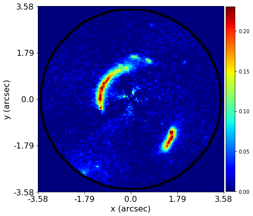
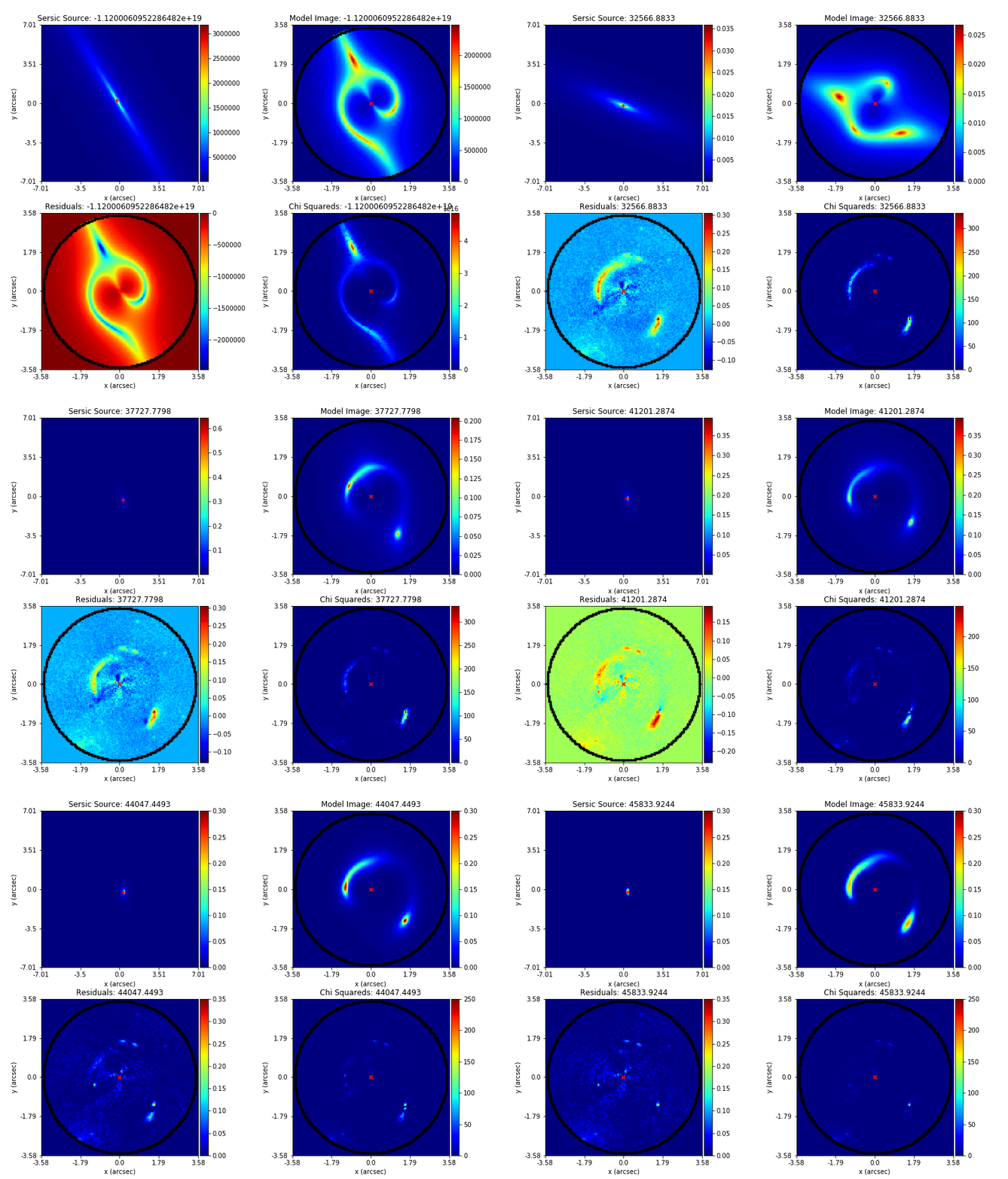
Here, we will see a concrete example of how PyAutoLens does it. It is a bit dense, but focus on the image on the right: this is your observed data, and it is an image of a strong gravitational lensing. The question to ask is, out of all those complicated parameters, how would you come up with a model that predicts exactly that pattern?
The animation shows how iterations of different parameters converge on that pattern.
At the start, the image in the top right hand corner does not really resemble the observation. But as it iterates more and more, it gradually becomes it. Eventually, comparing the image in the top right hand corner against the data, we can see the modeled image pretty much ressemble it.
Here is how we can infer on the mass of the dark matter we cannot see.
One more thing you can notice here is, while probably I can implement the likelihood function in any language I want, eventually I need to expose it in a Python interface because I need to pass it to these libraries: Nested sampling (Dynesty), MCMC (emcee), particle swarm optimization (PySwarms).
This is what I mean when I say the superpowers of Python is it is where the community is, and why which language we implement it does not matter. Python is still our favorite glue. With JIT in Python like Numba and JAX, we can stick to the glue a bit longer.
So, who won?
So in this particular case — PyAutoLens — who won the battle of JIT? Can you guess?
JAX, of course. Our project was funded to move things from Numba to JAX; if JAX had lost, we would basically be a complete failure. The interesting question is by how much. The room guessed five times.
It is 50x, according to preliminary results. On the slide that number is set fifty times larger than the text around it, which is roughly the point — I don’t feel good about the typography, but that is how much.
Team, Links, & References
- PyAutoLens Team
- James W. Nightingale
- Richard G. Hayes
- Aristeidis Amvrosiadis
- Coleman Krawczyk
- Gokmen Kilic
- …
- Link of this project: https://ickc.github.io/python-autojax/. This is a standalone framework to compare different implementations of functions. Functions are being upstreamed to PyAutoLens.
- Link to example used today
- For different ways to do reduced sum efficiently in JAX, see python-autojax/experiments/reduced_sum at main · ickc/python-autojax for more.
- Scientific Computing with JAX | Durham HPC Days
Lastly, I just want to point you to the team of people working on this and some links to share. Thank you.